
A Step-By-Step Guide: Unraveling the Magic of Store Segmentation with K-means Clustering in R

Introduction
As someone who works in retail and has the opportunity to teach what I get to explore in the industry, I often find myself fielding questions about store segmentation. "What's the ROI of the process?" "Which programming language is your go-to?" "Which algorithm tops your list?"
Well, let me show you, my friends!
Honestly, store segmentation emerges as a potent tool, a secret weapon that empowers manufacturers and retailers to dissect certain data and strategize with precision. By clustering stores with similar traits, retailers can delve into different segments and tailor their strategies accordingly.
In this blog post, we'll embark on a step-by-step journey through the process of performing store segmentation using a method that's as prevalent as it is powerful - K-means clustering using #Rcode and #Rstudio as my #IDE.
1) Why K-means, you ask? It's simple to implement, computationally efficient, and works like a charm for large datasets, making it a popular choice among data scientists.
2) Which data science language should I use? I prefer to use R. Honestly, it’s the most familiar and agile language for data science. However, Python is also more than capable and even more powerful when combining ML or unobserved analytic methodologies.
Step 1: Data Preparation
Every excellent data analysis project begins with preparing the data. We'll need data on various aspects of each store's performance for our store segmentation. Here's a sneak peek into how you might whip up a sample dataset in R:
This code conjures up a RANDOM data frame with 11 categories for each of the 250 stores, with various metrics for each category.
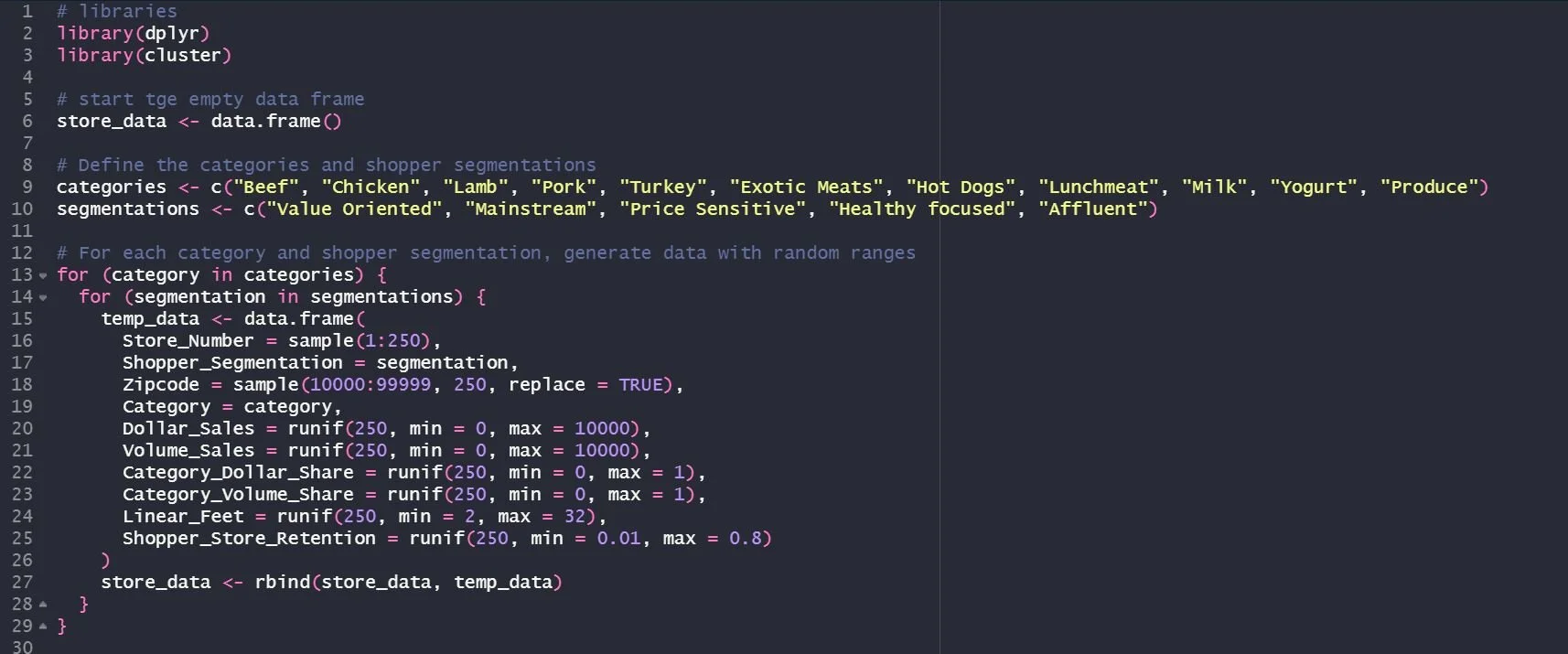
Step 1: raw code
Step 2: K-means Clustering & Breakdown
With our data ready and ready, we can dive into K-means clustering. This unsupervised machine learning algorithm groups data based on their similarity. In R, we can summon the kmeans function to perform K-means clustering:
This code selects only the numeric columns for clustering, performs K-means clustering with 5 clusters, and adds the cluster assignments to the original data. It's like magic but with code!

Now let’s break down what this code actually DOES!
numeric_data <- store_data %>% select(Dollar_Sales:Shopper_Store_Retention)
is using the select function from the dplyr package to select only the columns from Dollar_Sales to Shopper_Store_Retention in the store_data data frame. The %>% the operator is a pipe operator from the magrittr the box that is used to chain together multiple operations. The result of this operation is a new data frame numeric_data that contains only the selected columns.
Following line of code:
print(head(numeric_data))
Using the head function to display the first six rows of the numeric_data data frame. The print process is then used to print these rows to the console.
The output you're seeing is the first six rows of the numeric_data Data frame. Each row represents a store, and each column represents a different metric for that store. Here's a brief explanation of each column:
Dollar_Sales: The total sales for the store in dollars.Volume_Sales: The total sales for the store in volume (e.g., number of items sold).Category_Dollar_Share: The proportion of the store's total sales from a specific category in terms of dollars.Category_Volume_Share: The balance of the store's total sales from a specific type, in terms of volume.Linear_Feet: The amount of shelf space allocated to a particular category in the store, measured in linear feet.Shopper_Store_Retention: The proportion of shoppers who return to the store.
By examining these measures, you can START to gain insights into the performance of each store and each category within each store. For example, a high Category_Dollar_Share for a specific type might indicate that this category is a significant driver of sales for the store.
Step 3: Analyzing the Clusters
Once we've conjured up the clusters, we can analyze them to understand their characteristics. Here's how you might calculate the cluster centers and the distribution of stores in each cluster:
This code calculates the cluster centers, which are the average values of each variable for the stores in each cluster, and counts the number of stores in each cluster. It's like getting to know each cluster personally!
WHY KMEANS?!
K-means clustering is a popular choice for segmentation tasks due to its simplicity, efficiency, and ease of interpretation. Here are some reasons why we might choose K-means over other segmentation methods:
Simplicity: K-means is a straightforward algorithm that is easy to understand, even for beginners. It doesn't require any advanced statistical knowledge to interpret the results.
Efficiency: K-means is computationally efficient, especially for large datasets. This is because the algorithm only needs to calculate the distances between data points and cluster centers, which can be done quickly.
Flexibility: K-means can be applied to any type of continuous data, not just data that follows a specific distribution. This makes it a versatile tool for many different segmentation tasks.
Visualization: The results of K-means clustering can be easily visualized, especially when the data has two or three dimensions. This can help to intuitively understand the segmentation results.
Scalability: K-means can handle large datasets and high dimensional data, making it suitable for many real-world applications.

Raw code
Code:
print(kmeans_result)
Is printing the results of the K-means clustering algorithm. The output provides a summary of the K-means clustering results, including:
The number of clusters and their sizes.
The group means the average values of each variable for the stores in each cluster.
The clustering vector, which shows the cluster assignment for each store.
The within-cluster sum of squares by cluster is a measure of the compactness of the clusters. Smaller values indicate that the points in a cluster are closer to each other.
The percentage of the total variance is explained by the between-cluster variance, which is a measure of the separation of the clusters. Larger values indicate that the clusters are more distinct from each other.
Following line of code:
store_data$Cluster <- kmeans_result$cluster
is adding the cluster assignments to the original store_data data frame. The $ operator is used to accessing the cluster component of the kmeans_result object, which is a vector of cluster assignments. The <- operator is used to assigning this vector to a new column cluster in the store_data data frame.
Last line of code:
print(head(store_data))
is using the head function to display the first six rows of the store_data a data frame, which now includes the cluster column. The print the function is then used to print these rows to the console.
The output you're seeing is the first six rows of the store_data data frame, with the cluster column added. Each row represents a store, and each column represents a different metric for that store or the cluster assignment. By examining these metrics and the cluster assignments, you can gain insights into the performance of each store and how stores are grouped into clusters based on their performance. For example, stores in the same set have similar values for the metrics, indicating that they have identical performance characteristics.

Step 3: Cluster Output
Step 4: Visualizing the Clusters
Visualizing the clusters can help us better understand the results. Because we have multiple dimensions in our data, we can use Principal Component Analysis (PCA) to reduce the dimensionality of the data to two dimensions, which can then be plotted:
This code performs PCA on the numeric data, adds the cluster assignments to the PCA results, and creates a scatter plot of the first two principal components, colored by cluster. It's like painting a picture with data!
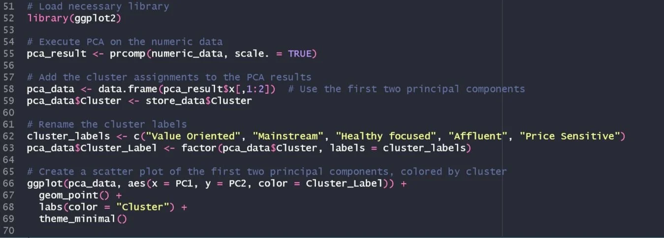
raw code
BREAKDOWN THE CODE!
library(ggplot2): This line loads the ggplot2 library, which is a powerful tool for creating professional quality plots in R.pca_result <- prcomp(numeric_data, scale. = TRUE): This line performs Principal Component Analysis (PCA) on the numeric data. PCA is a technique used to emphasize variation and bring out strong patterns in a dataset. It's often used to make data easy to explore and visualize. Thescale. = TRUEargument standardizes each variable to have a mean of zero and standard deviation of one, which is necessary when the variables are measured in different units.pca_data <- data.frame(pca_result$x[,1:2]): This line creates a new data frame that contains the first two principal components from the PCA result. These two components are the ones that explain the most variance in the data.pca_data$Cluster <- store_data$Cluster: This line adds the cluster assignments to the PCA results. Each store is assigned to the cluster that it was grouped into during the K-means clustering process.cluster_labels <- c("Value Oriented", "Mainstream", "Healthy focused", "Affluent", "Price Sensitive"): This line creates a vector of cluster labels.pca_data$Cluster_Label <- factor(pca_data$Cluster, labels = cluster_labels): This line assigns the descriptive labels to the clusters in the PCA data.The last block of code creates a scatter plot of the first two principal components, with points colored by cluster. The
geom_point()function adds points to the plot (one for each store), theaes(x = PC1, y = PC2, color = Cluster_Label)part sets the x and y coordinates of the points to the first and second principal components, and colors the points by cluster. Thelabs(color = "Cluster")part sets the label for the color legend to "Cluster", andtheme_minimal()sets a minimalistic theme for the plot.

Let’s analyze the clusters:
Value Oriented: This cluster represents stores that are likely attracting customers who are looking for the best value for their money. These customers are not necessarily looking for the cheapest products, but rather products that offer the most bang for their buck. The stores in this cluster might have a wide variety of products and offer many deals and promotions.
Mainstream: Stores in this cluster are likely to have a broad appeal to a wide range of customers. They might carry a mix of products to cater to different customer segments. These stores might be located in densely populated areas and could be large chain stores.
Healthy Focused: These stores are likely to attract health-conscious customers. They might be offering a wide range of organic, gluten-free, vegan, and other health-oriented products. These stores might also have a fresh produce section and could be located in neighborhoods where customers are more health-conscious.
Affluent: Stores in this cluster are likely located in affluent neighborhoods and cater to customers with a higher disposable income. They might carry high-end, luxury, and gourmet products. These stores might offer a superior shopping experience with excellent customer service.
Price Sensitive: This cluster represents stores that attract price-sensitive customers. These customers are likely to be very conscious of prices and are always looking for the best deals and discounts. These stores might carry more generic or store-brand products and might have frequent sales.
Remember, this is a hypothetical analysis based on the cluster labels we've assigned. The actual characteristics of the clusters would depend on the ACTUAL SYNDICATED DATA used for clustering.
Conclusion
Store segmentation is a powerful tool in retail analytics, and K-means clustering is a simple yet effective method for performing store segmentation. By grouping stores based on similar characteristics, retailers can gain insights into different segments and tailor their strategies accordingly. With the power of R and the K-means clustering algorithm, retailers can leverage their data to make informed decisions and drive their business forward. It's like having a secret weapon in your retail arsenal!